
Create a Recommendation Engine with AI for Free
24th March 2025 • 6 min read — by Aleksandar Trpkovski
Recently, I had some free time since I was taking a month off work for the arrival of my daughter. While at home, I decided to make some updates to my personal blog.
Previously, my blog displayed three recommended articles at the bottom of each post. These articles were simply the next consecutive ones, which was easy to implement and required no AI or complex algorithms. For example, if an article was written on March 2, 2025, the recommended articles would be from January 15, January 9, and January 4, since these were the three most recently published articles before the current one. See image below
However, these recommendations weren't very relevant—readers rarely found articles that matched their interests.
In this article, I'll walk you through exactly how I did it—for free—using open-source AI models to make article suggestions more relevant for readers. Let's dive in!
What Are Embedding Models and Why Do We Need Them?
Before we dive into the implementation, let's first understand embedding models and why they are essential for building a recommendation system.
At a high level, embedding models are AI models that convert text into numerical vectors—essentially transforming words, sentences, or even entire articles into numbers that a computer can understand. These vectors help capture the meaning and relationships between different pieces of text.
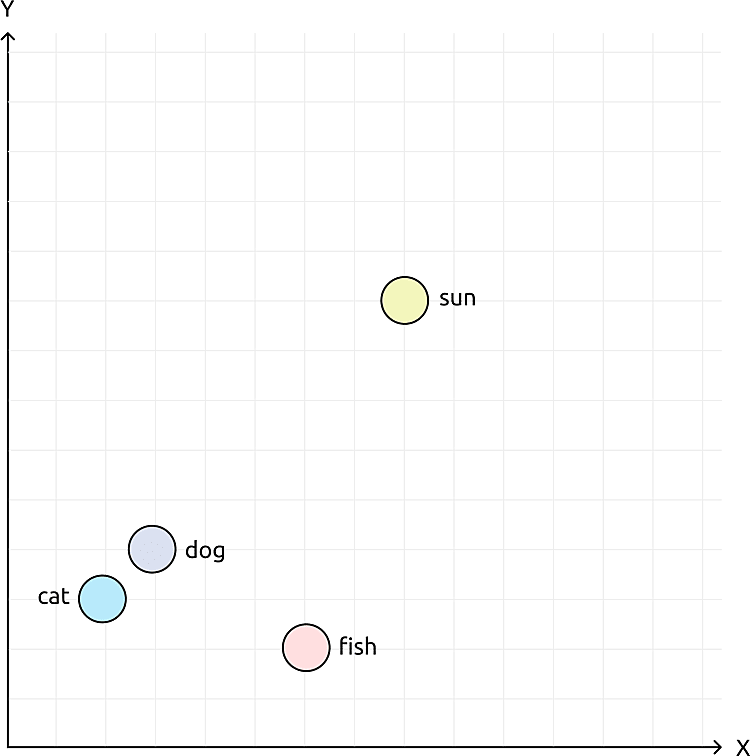
For example, imagine we want to represent words in a 2D space where similar words are close together. An embedding model can do this. Take the words cat, dog, fish, and sun. We can represent them with vectors like this: cat becomes [2, 3], dog [3, 4], fish [6, 2], and sun [8, 9]. Here, cat and dog are close because they are both animals, while fish is further away (another animal but different category), and sun is very far because it's unrelated.
In the context of our recommendation system, embeddings allow us to measure the similarity between articles. Instead of just suggesting the next article in order, we can recommend articles that are most relevant to what the reader is currently viewing.
Paid vs. Free Embedding Models
There are many different embedding models available, and they generally fall into two categories:
Paid Embedding Models (e.g., OpenAI, VoyageAI, Google)
The major AI companies like OpenAI, VoyageAI, and Google provide embedding models.
OpenAI offers high-quality embedding models, such as text-embedding-3-large, text-embedding-3-small, and text-embedding-ada-002.
VoyageAI's options include voyage-3, voyage-3-large, and voyage-3-lite.
Google provides text-embedding-004 and text-embedding-005.
Since these models charge API usage fees, they aren't ideal for small projects or personal blogs.
Free Embedding Models (e.g., Hugging Face)
Fortunately, there are open-source alternatives that are completely free! Hugging Face is a popular platform that hosts a wide range of pre-trained AI models, including embedding models. Many of these models can be used without any cost, making them perfect for personal projects like ours.
For this tutorial, we will use a free embedding model from Hugging Face. This allows us to build a zero-cost recommendation system while still leveraging the power of AI.
Understanding Embedding Dimensions and Sizes
In the world of embedding models, "dimensions" or "sizes" refer to the number of numerical values (or "coordinates") used to represent text in a numerical space.
Remember our earlier example with two-dimensional coordinates (x, y)? Embedding models work the same way but use hundreds or thousands of dimensions instead of just 2 or 3.
More dimensions allow the model to capture finer nuances and relationships between words and concepts—like having a more detailed meaning map. Fewer dimensions create a simpler representation, which produces a smaller numerical representation (the "embedding"). Higher dimensions offer better accuracy but require more storage and computing power.
For example, OpenAI and VoyageAI offer various types of embedding models. Their larger models like text-embedding-3-large and voyage-3-large use 3072 and 2048 dimensions respectively, while their lighter models like embedding-3-small and voyage-3-lite use as few as 512 dimensions.
Using Hugging Face and Transformer.js
For my blog article, I decided to use a free recommendation engine by leveraging the power of Hugging Face and Transformer.js.
What is Transformer.js?
Transformer.js is a JavaScript library that lets you run AI models directly in your web browser or Node.js application. It downloads models locally, allowing them to run entirely on your device.
It supports various models including text generation, translation, image recognition, and embedding generation—all without relying on external APIs. This means zero usage fees, making it ideal for my personal blog project.
Choosing the Right Model
Since the models in Transformer.js run locally, we need to be mindful not to choose a model that's too large in size and requires significant computing power to generate embeddings. For that purpose, I chose a model called all-MiniLM-L6-v2.
This model converts sentences and paragraphs into 384-dimensional dense vector embeddings, providing an excellent balance of performance and efficiency.
For compatibility with Transformers.js, I use the Xenova/all-MiniLM-L6-v2 model from Hugging Face.
Implementing the Embedding Extraction
First, let's install the @huggingface/transformers package:
npm install @huggingface/transformers
Here's the simple code to compute embeddings from text:
import { pipeline } from "@huggingface/transformers";

const text = "The Importance of Machine Learning in Modern Web Development";

const extractor = await pipeline("feature-extraction", "Xenova/all-MiniLM-L6-v2");
const output = await extractor(text, { pooling: "mean", normalize: true });
const vector = output.tolist();
console.log(vector[0]);
The console log from the above code will output the following 384-dimensional vector:
[
   -0.020516404882073402,   -0.00818917341530323,    0.02859281376004219,
    0.039169277995824814,    0.07049212604761124,   -0.02238479070365429,
    -0.03139492869377136,   -0.06332399696111679,   -0.04767751693725586,
    -0.02019294537603855,   -0.05919709429144859,    0.04298273101449013,
    0.016094526275992393,    -0.0438438318669796,  -0.024306558072566986,
     0.01921924203634262,  -0.028016094118356705,   -0.03439173847436905,
    -0.04121260717511177,   -0.10778705775737762,  -0.021788278594613075,
    -0.03216289356350899,    0.01833938993513584,  -0.017994459718465805,
  0.00037811059155501425,    0.04635584354400635,   0.019866760820150375,
     0.05040336400270462,    0.06332680583000183,   -0.03538951650261879,
   -0.005023809149861336,    -0.0143986064940691, -0.0052444711327552795,
    0.023529207333922386,   -0.07226388156414032,    0.07632710039615631,
     0.01021984126418829,   -0.00824225414544344,    0.03339964896440506,
    -0.01060909777879715,   -0.09655245393514633,  -0.055546682327985764,
   -0.012066159397363663, -0.0076921964064240456,    0.04580942541360855,
     0.02390001341700554,   -0.08683866262435913,   -0.08001071214675903,
     -0.0641876757144928,   0.017844615504145622,   -0.08620015531778336,
    -0.08266746997833252,   0.022476131096482277,  -0.036314111202955246,
    -0.06440844386816025,     0.0329846553504467,    0.03954195976257324,
    -0.02818935364484787,   0.016931047663092613, -0.0027509541250765324,
   -0.012003917247056961,   -0.08396296203136444,   0.020469816401600838,
    0.007711503189057112,   0.039566002786159515,  -0.023063624277710915,
   -0.001518305274657905,    0.03386910259723663,  -0.005670216400176287,
     0.01568906381726265,    -0.0874529480934143,     0.0704861655831337,
    -0.08309027552604675,    0.06774929165840149,  -0.013879545032978058,
    -0.03932321444153786,  -0.026192566379904747,  0.0037247256841510534,
    0.025735696777701378,   0.042777273803949356,  -0.006177722010761499,
    0.016913456842303276,  -0.019507644698023796,    0.07432487607002258,
    0.043784961104393005,    0.03311076760292053,   0.005122023168951273,
   -0.019937295466661453,  -0.058375801891088486,   -0.07924377918243408,
   -0.015307264402508736,  -0.026857662945985794,    0.04473648965358734,
   -0.003576496383175254,   -0.03769933804869652,   0.016773588955402374,
    0.008591416291892529,   -0.07192342728376389,   -0.03686879947781563,
     0.09621886163949966,
  ... 284 more items
]
At first glance, these numbers might look meaningless, but trust me—we'll see later how these numbers help us compare vectors of different texts to determine their similarity. But before that, let's see what each part of the code above does:
- Load a Feature Extraction Model – The
pipelinefunction loads theXenova/all-MiniLM-L6-v2model. It downloads once and caches locally, making subsequent runs faster. - Process the Text – The extractor converts the input text (
"The Importance of Machine Learning in Modern Web Development") into a 384-dimensional vector. - Pooling & Normalisation – The
pooling: "mean"option averages the token embeddings, whilenormalize: trueensures consistent scaling. - Convert to Array & Output – The resulting vector is converted to an array and logged to the console.
Calculate cosine similarity between two embeddings
Now that we have extracted embeddings from a single text, let's compare the similarity between two different texts using cosine similarity. Cosine similarity is a common metric for measuring the similarity between two vectors, with a value between -1 (completely opposite) and 1 (identical).
For calculating the cosine similarity, we'll use a helper library for Node.js from TensorFlow called @tensorflow/tfjs-node. First, we need to ensure we have this package installed:
npm install @tensorflow/tfjs-node
Compute Embeddings for Two Texts
import { pipeline } from "@huggingface/transformers";
import * as tf from "@tensorflow/tfjs-node";

// Define two different texts
const text1 = "The Importance of Machine Learning in Modern Web Development";
const text2 = "Machine learning is transforming the future of web applications.";

// Load the feature extraction model
const extractor = await pipeline("feature-extraction", "Xenova/all-MiniLM-L6-v2");

// Extract embeddings for both texts
const output1 = await extractor(text1, { pooling: "mean", normalize: true });
const output2 = await extractor(text2, { pooling: "mean", normalize: true });

const vector1 = output1.tolist();
const vector2 = output2.tolist();
Compute Cosine Similarity
// Function to calculate cosine similarity
function cosineSimilarity(vec1, vec2) {
    const dotProduct = tf.sum(tf.mul(vec1, vec2));
    const magnitude1 = tf.norm(vec1);
    const magnitude2 = tf.norm(vec2);
    return dotProduct.div(magnitude1.mul(magnitude2)).dataSync()[0];
}

// Calculate similarity
const similarityScore = cosineSimilarity(vector1, vector2);
console.log("Cosine Similarity Score:", similarityScore);
Understanding the Results
The cosine similarity score indicates how semantically similar two texts are. A score closer to 1 means the texts are very similar, while a lower score indicates they are less related.
For example, from above the output will be like:
Cosine Similarity Score: 0.787977933883667
This indicates that the two texts are quite similar in meaning. If we compared completely different topics, the score would be much lower, like 0.2 or 0.3.
Similar Article Suggestions in My Blog
Now that we understand how to generate embeddings and calculate cosine similarity, let me show you how I implemented this in my personal blog. Built with Nuxt.js and the Nuxt Content module, my blog stores articles in Markdown format, providing a structured way to access and process content.
The first step was extracting textual content from all blog articles' Markdown files. During static site generation, I used the embedding extraction code we discussed earlier to generate a numerical vector representation for each blog post.
With all articles converted to numerical vectors, the next step was determining article similarity. When someone reads a blog post, my system calculates the cosine similarity between that article's vector and all other articles' vectors. This reveals which articles are most semantically related.
I then select the three articles with the highest cosine similarity scores. These closest content matches appear at the bottom of the current article as reading suggestions.
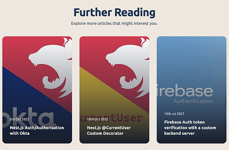
For example, when a user reads an article about Nest.js Authorisation with Firebase Auth, they'll see suggestions for: Nest.js Auth/Authorisation with Okta, Nest.js @CurrentUser Custom Decorator, Firebase Auth token verification with a custom backend server
For those interested in seeing the implementation details, the complete source code of my blog is available on GitHub here.
The example above is available on this repository here.
Further Reading
Explore more articles that might interest you.